A gut microbial signature for

CA209-538: clinical trial procedures

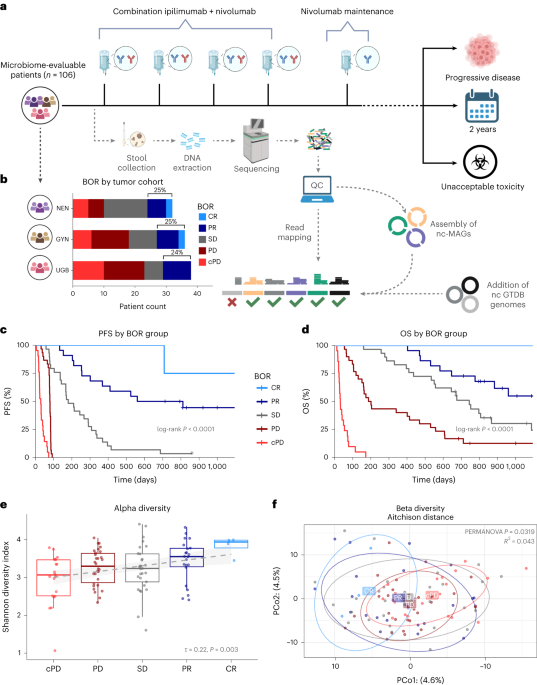
CA209-538, titled ‘A phase 2 trial of ipilimumab and nivolumab for the treatment of rare cancers’, is an investigator-initiated, prospective, multicenter, single-arm clinical trial (NCT02923934). The study was approved by the Austin Health (Melbourne, Australia) Human Research Ethics Committee (approval: HREC/16/Austin/152).

Between October 2017 and February 2020, 120 adult patients with rare cancers were recruited across five sites in southeastern Australia (Austin Health, Peter MacCallum Cancer Centre, Monash Health, Blacktown Hospital and Albury Wodonga Health/Border Medical Oncology). Patients were recruited into three prespecified ‘histology cohorts’ of approximately equal sizes: (1) UGB, comprising cholangiocarcinomas, gallbladder cancers, duodenal cancers and gastrointestinal stromal tumors; (2) NEN, including neuroendocrine tumors or carcinoma of any primary organ (except small cell lung carcinoma) or adrenocortical carcinoma; and (3) GYN, comprising diverse histologies including carcinosarcoma, low-grade serous carcinoma and clear-cell carcinoma of gynecological organs.

Patients were eligible if they had a histologically confirmed diagnosis of a target rare cancer (UGB, NEN or GYN cancers) that was advanced or metastatic, an Eastern Cooperative Oncology Group (ECOG) performance status of 0–1, a measurable tumor lesion per RECIST 1.1 criteria61 and screening blood laboratory values largely within normal limits. Prior systemic therapy or radiotherapy was permitted if completed at least 4 or 2 weeks, respectively, of the first administration of the study drugs and all related adverse events had stabilized or returned to baseline. The exclusion criteria included active central nervous system metastases (brain or leptomeningeal); prior CICB (monotherapy was permitted); prior malignancy active in the previous 3 years; active, known or suspected autoimmune conditions; and requirement for systemic corticosteroids >10 mg prednisolone daily or equivalent. Participants provided fully informed written consent, including for the collection and analysis of biospecimens (including fecal samples) and sharing of anonymized data as part of research collaborations. The data cutoff was May 7, 2022, providing a minimum of 26 months of follow-up for all participants.

All patients were intended to be treated with CICB in the form of nivolumab 3 mg kg−1 and ipilimumab 1 mg kg−1 three weekly for four doses (induction), followed by nivolumab monotherapy maintenance (3 mg kg−1 two weekly or 480 mg four weekly after a protocol amendment) for up to 2 years or until PD or unacceptable toxicity. The trial’s prespecified primary endpoint was to determine the clinical efficacy of CICB in patients with rare cancers using the RECIST 1.1 BOR61. In brief, BOR was determined at data cutoff and defined as the investigator-assessed RECIST 1.1 best response designation at any on-trial time point until the date of objectively determined progression per RECIST 1.1 or the date of subsequent anticancer therapy commencement. For participants without documented progression or subsequent therapy, all available response designations contributed to their BOR assessment. The trial’s minimum duration criterion for the determination of SD was 9 weeks.

For the assessment of radiographic response, all patients were intended to undergo whole-body cross-sectional imaging with computed tomography or magnetic resonance imaging at baseline (within 28 days before registration), 12 weeks, 18 weeks and then 12 weekly thereafter (±1 week). Patients with rapid disease-related clinical deterioration who were thus unable to undergo restaging imaging at the first restaging time point were deemed to have cPD. PFS and OS were determined from the date of first treatment; the efficacy and safety outcomes for various trial subcohorts have been reported previously23,24,25,26. Given the accumulating evidence of ‘pseudoprogression’ in a minority of ICB recipients62, under the trial protocol, ICB therapy could extend beyond RECIST 1.1-defined PD if there was investigator-assessed clinical benefit and good participant tolerance of the study drugs until there was evidence of a further 10% or greater increase in target lesion dimensions or further new disease sites.

Other clinical metadata

Detailed information on tumor characteristics, demographic factors, blood laboratory values and concomitant medications was collected by the site investigators into an electronic case report form. For this analysis, we included the following 15 clinical metadata variables, as we hypothesized their potential relevance to treatment response and/or gut microbial compositions based on our literature review: patient age (years, at time of trial commencement), sex, body mass index, ECOG performance status, histology cohort (based on the pathology report), extent of measurable tumor (based on the sum of RECIST target lesion diameters calculated using the computed tomography scan at trial screening), study site, season of fecal sample collection, antibiotic use, proton-pump inhibitor use, chemotherapy use, blood NLR, platelet count, albumin levels and lactate dehydrogenase levels (Supplementary Table 3). Only one participant had received prior ICB monotherapy (a NEN cohort patient treated with anti-PD-1 therapy ceased 20 months before trial treatment); given that only one patient was involved, this was not included as a clinical variable. Antibiotic, proton-pump inhibitor and chemotherapy use was defined as their recorded use within the 8 weeks before cycle 1 of study treatment, given the evidence of antibiotic perturbations of gut microbial compositions lasting this duration63. The different antibiotics used were amoxicillin, amoxicillin plus clavulanic acid, ampicillin, azithromycin, cefalexin, cefazolin, ceftriaxone, clindamycin, co-trimoxazole, doxycycline, flucloxacillin, gentamicin, norfloxacin, penicillin, piperacillin plus tazobactam and metronidazole. As only 9 of the 106 microbiome-evaluable patients had used any antibiotics in this 8-week period, they were not further subcategorized based on class or antimicrobial coverage. The different proton-pump inhibitors used were esomeprazole, pantoprazole, rabeprazole and omeprazole.

Fecal sample collection

The collection of fecal samples was added to the study protocol in version 5 (July 24, 2017). Participants were trained and provided OMR-200 ‘OMNigene GUT kits’ (DNA Genotek) to collect a fecal sample immediately before treatment (from day −7 to day 0 relative to cycle 1 of trial treatment). OMR-200 kits are designed to stabilize DNA and have been shown to enhance DNA quantifications and stability across storage temperatures relative to nonpreservative alternatives64. Fecal samples were express-shipped to the Olivia Newton-John Cancer Research Institute, where they were then frozen at −80 °C for long-term storage. DNA was extracted using the FastDNA kit (MP Biomedicals), including a negative control using ultrapure water. DNA samples were shipped to the Wellcome Sanger Institute on dry ice for shotgun metagenomic sequencing.

Fecal shotgun metagenomic sequencing and analysis

DNA sequencing and quality control

DNA samples were quantified using a Qubit fluorometer, and whole metagenome libraries were deeply sequenced on a single run of the NovaSeq 6000 S4 platform (2 × 150-bp paired-end reads), generating a median of 20,477,028 raw paired-end reads per sample (interquartile range 19,244,530–22,056,539 paired-end reads). Raw sequencing data were first human decontaminated by the Wellcome Sanger Institute core sequencing team by removing read pairs in which one or both aligned to the GRCh37 human genome assembly using bwa (v0.7.17; ‘aln’ then ‘sampe’ commands)65. These data were further quality controlled using the metaWRAP (v1.2)66 ‘reads_qc’ pipeline, which first trimmed low-quality bases using trim-galore (v0.6.7)67 (default parameters) and then performed a second pass of human decontamination with BMTagger (v3.101)68 using the GRCh38 human genome assembly. Finally, a median of 20,359,318 clean paired-end reads per sample (interquartile range 19,014,843–21,771,873) were available for further analysis.

MAG assembly

Quality-controlled paired-end reads were first assembled individually with SPAdes (v3.14) using option ‘-meta’ (refs. 69,70). Unassembled reads were then recovered by mapping raw reads back to metaSPAdes-assembled contigs using bwa ‘mem’ (v0.7.17)65, followed by reassembly with MEGAHIT (v1.2.4)71 using default parameters. Subsequently, the sample-wise metaSPAdes and MEGAHIT assemblies were combined and sorted, with short contigs (<1,500 bp) removed. The resulting assemblies were then independently binned with MetaBAT 2 (v2.13)72, MaxBin2 (v2.2.4)73 and CONCOCT (v0.4)74 using default parameters and a minimum contig length threshold of 1,500 bp (option ‘–minContig 1500’). The depth of contig coverage required for the binning was inferred by mapping the raw reads back to their assemblies with bwa-mem and then calculating the corresponding read depths for each contig with samtools (v1.5)75 (‘samtools view -Sbu’ followed by ‘samtools sort’), together with the ‘jgi_summarize_bam_contig_depths’ function in MetaBAT 2.

Thereafter, individual bin sets produced by the three binning programs were consolidated into a refined bin set consisting of the best version of each bin based on the most optimal genome completion and contamination metrics among all seven versions of hybridized bin sets (MetaBAT 2, MaxBin2, CONCOCT, MetaBAT 2 + MaxBin2, MetaBAT 2 + CONCOCT, MaxBin2 + CONCOCT, MetaBAT 2 + MaxBin2 + CONCOCT), as estimated by CheckM (v1.1.2)76 using the metaWRAP (v1.2) ‘bin_refinement’ pipeline66. Finally, the final bin sets were further improved by performing reassembly with SPAdes in ‘–careful’ mode after both strict and permissive mapping of raw reads and keeping the bin sets with the best CheckM metrics. In total, 4,277 MAGs with ≥50% completion and ≤5% contamination were generated. These were then further quality controlled, now for ≥90% completeness and ≤5% contamination using CheckM2 (v0.1.3)77 and for strain-level contamination using GUNC (v1.0.5)78 to finally identify 2,209 quality-controlled nc-MAGs consistent with the MIMAG (minimum information about a MAG) criteria79. Finally, study-specific MAGs were taxonomically classified (using GTDB r207 taxonomy) with GTDB-tk (v2.1)80, pplacer (v1.1)81 and fastANI (v1.3)82.

Generation of a custom, MAG-informed reference database

As the recovery of MAGs may be challenging for some (for example, low abundance or difficult to assemble) strains, we sought to supplement our study-specific strain genome reference database with SRGs from GTDB r207 (62,291 bacterial and 3,412 archaeal genomes) to create a ‘hybrid’ reference library. To identify a relevant shortlist of GTDB SRGs, we first mapped quality-controlled reads from our study to the full GTDB r207 SRG database with Bowtie 2 (v2.3.5)83 and inStrain (v1.3.0)84 (using default settings in ‘–database’ mode). After further filtering of reads mapped to <0.5 SRG breadth, we determined that n = 1,076 SRGs were present. We combined these SRGs with the study-specific nc-MAGs (total 3,285) and used dRep (v2.0.0)85 to dereplicate the combined genome set to 98% identity using the settings ‘-comp 90 -con 5 –S_algorithm fastANI –S_ani 0.98 –cov_thresh 0.50 –multiround_primary_clustering –greedy_secondary_clustering’. An absolute nucleotide identity (ANI) threshold of 98% was chosen as a compromise between offering subspecies (strain-level) resolution for read classification while still mitigating ‘read stealing’ due to overly similar reference genomes (as detailed in the inStrain documentation). Ultimately, n = 1,397 genomes were selected using dRep and formed our ‘hybrid’ custom strain reference database. Of these, just over half were study-specific nc-MAGs (714, 51%), whereas the remainder were either near-complete isolate (423, 30%) genomes or nc-MAG (260, 19%) SRGs. Using GTDB-tk, we could classify 1,363 of the 1,397 genomes to 904 separate GTDB r207 species clusters (898 bacteria, 6 archaea), with the remaining 34 (32 bacteria, 2 archaea) representing completely new species. For the 904 ‘known’ species, 705 species had 1 strain, whereas 199 species had 2–21 strains each. The species with n = 21 distinct strains by 98% ANI delimitation was Ruminococcus D bicirculans (Supplementary Table 16).

Read mapping to a custom strain database

We first used Bowtie 2 to generate a mapping index and then to align reads to our custom reference database. We then used the inStrain profile, now with settings ‘–min_read_ani 0.95 –min_genome_coverage 1’, to perform more precise quality control of the mapped reads. InStrain uses information on paired-end read orientation, mapQ score, insert size and ANI value to filter read mappings stringently, resulting in high-confidence quantifications.

To enhance our confidence about read mappings further, we removed reads mapped with <0.5 genome breadth coverage, as low genome breadth might indicate mapping to mobile genetic elements or mismapping. For our discovery cohort, a median of 50% (range 39–73%) of quality-controlled reads were ultimately used for abundance estimation of strains within each sample (Supplementary Fig. 1).

We finally used Decontam (v1.16.0)86 to screen for potential contaminants. Reassuringly, after the above steps, no bacteria were identified in our negative control sample for the discovery cohort. Based on the ‘frequency’ method (inverse correlation between the abundance of strains and the DNA concentration of submitted samples), one strain was identified as a potential contaminant in over 10% of samples from our discovery cohort (CA209-538 cohort) and was thus removed (Pseudomonas E sp002874965; Supplementary Fig. 4).

Downstream analysis of taxonomic abundances

Most downstream microbiome analyses were performed in the R (v4.1.0) environment, using ‘phyloseq’ (v1.12.0)87, ‘microbiome’ (v1.12.0)88 and ‘vegan’ (v2.6.4). Specifically, alpha diversity was computed using the Shannon diversity index on strain relative abundances (each sample’s sum abundances transformed to a sum of 1). As we found no association between the Shannon diversity index and clean paired-end reads in our discovery cohort (Pearson R = 0.068, P = 0.49), we did not perform rarefaction. Beta diversity was calculated using the strain Aitchison distance, a measure of Euclidean distance of CLR-transformed abundances, computed using log(a/gma), where a is the species relative abundance and gma is the sample geometric mean relative abundance (with a small pseudocount of one-half the minimum nonzero abundance added to all values to account for zeros). As CLR abundances may better account for the inherent compositionality of microbial abundance data89, CLR-transformed feature abundances were exclusively used for the supervised ML analyses.

Generation and visualization of phylogenetic trees

For whole bacterial kingdom genome sets, approximately maximum-likelihood phylogenetic trees were constructed using GTDB-tk (v2.1.0)80 (aligning 120 ubiquitous bacterial genes) and FastTree (v2.1.0)90 using the WAG model (Fig. 3a,b). For the tree of Faecalibacterium genomes, pairwise whole-genome ANI distances were computed using FastANI82 (many-to-many mode), which was converted into a distance matrix and then to a Newick-format tree using rapidNJ (v2.3.3)91 (Supplementary Fig. 2). Trees were visualized using the R package ggtree (v3.2.1)92.

Functional annotation

To evaluate the presence of virulence factor genes, we used abricate (v1.0.1)93 to screen relevant strain genomes against the VFDB (Virulence Factor Database)94. To profile strain metabolic potential broadly, we used gapseq (v1.2)95 using the ‘gapseq find’ command with default settings. Briefly, this involved performing a homology search of genomes (using TBLASTN (https://doi.org/10.1186/1471-2105-10-421)) for 28,768 reactions from 2,910 metabolic pathways (curated from MetaCyC and manually). Metabolic pathways were deemed present if ≥80% complete (lowered to ≥67% if ‘key’ reactions were present).

To evaluate butyrate production potential specifically, we used a previously validated multilevel approach involving hidden Markov models (HMMs)44,96. Briefly, we used a published database of 1,716 genomes and 19,284 genes to build HMM profiles (using HMMER v3.2.1; http://hmmer.org/) for the six genes encoding the acetyl-CoA butyrate-producing pathway (responsible for butyrate production through carbohydrate degradation). These genes are acetyl-CoA acetyltransferase (thl), β-hydroxybutyryl-CoA dehydrogenase (bhbd), crotonase (cro), butyryl-CoA dehydrogenase (bcd), and the alternative terminal enzymes butyryl-CoA:acetate CoA transferase (but) and butyrate kinase (butk). We then used these models to screen the strain genomes for the presence of these respective genes. As an orthogonal approach, we also mapped cleaned sample paired-end reads to the above genes’ sequences using Bowtie 2 and then used inStrain ‘quick profile’ to count mappings to estimate their sample-wise gene abundance (normalized per million reads) agnostic of source strain. The output is available in Supplementary Tables 13 (strain_top22_acetylcoa_pwy) and 14 (sample_acetylcoa_pwy).

Supervised ML analysis

Supervised ML analyses were performed in the Python 3 environment using the packages sklearn (v1.1.1)97, imblearn (v0.9.1)98 and their dependencies. The supervised ML pipeline involved a preprocessing step before model training and testing, performed separately for each training and testing instance to ensure no data leakage. This involved standard-scaling numerical features (computed using the formula z = (x − u)/s, where x is the feature value (for example, the CLR-transformed strain abundances), u is the mean of the fold samples and s is the s.d. of the fold samples) and one-hot encoding categorical features. Subsequently, only before classifier training (but not testing), classes of the target variable (RvsP or PFS12) were balanced with random oversampling with replacement.

We chose to use RF as our classifier, given its, on average, superior performance using microbial feature sets in previous benchmarking studies31. RF uses bootstrapped data to create an ensemble of decision trees (each trained on a subset of features), with the ultimate classification based on consensus; thus, it is feature scale invariant and able to capture nonlinearities and is also interpretable using TreeSHAP (described subsequently).

Our hyperparameter tuning procedure involved a random hyperparameter search over a broad array of options with 1,000 separate combinations tested, aiming to maximize the ROC AUC averaged over 20 times repeated fivefold cross-validation (that is, 100 separate models trained and tested (splits), for each 1,000 iterations, for each feature and classifier combination).

ROC AUC is a popular classifier performance metric that evaluates the discriminative performance across all potential decision thresholds, thus allowing for a head-to-head comparison of differently calibrated classifiers99. Ultimately, the best hyperparameter combination (based on mean AUC) was selected and referred to as the ‘tuned’ pipeline. The optimal hyperparameters and AUC scores for all 100 splits for all full feature sets are listed in Supplementary Table 9 (hyperparam_tuning_all).

To evaluate model performance, we used cross-validation (for example, leave-one-histotype-out cross-validation) or completely separate training and test cohorts (for example, training a model using one study cohort and then testing the fitted model on another cohort). Whenever evaluating model performance, training and testing procedures were repeated 100 times, and the resultant predictions were averaged to account for the stochasticity of our RF pipeline. As with hyperparameter tuning, ROC AUC was our metric of choice for gauging model performance.

Feature importances were evaluated with the ‘shap’ package using the TreeExplainer() function. Based on the foundation of game theory, TreeExplainer computes the influence of each feature (strain abundance) in determining the RF classifier’s local (per-sample) prediction. Therefore, we computed global feature importances (cohort-wide average of the absolute TreeExplainer scores) and imputed the importance ‘direction’ (that is, positive or negative influence on response prediction) by constructing a simple linear model between the feature values and SHAP values. We repeated this procedure 1,000 times to account robustly for the RF pipeline’s stochasticity. The global feature importance and s.d. values of all features are listed in Supplementary Table 12 (strain_importance).

Literature review and meta-analysis of relevant published datasets

We sought to identify all published clinical datasets that met the following criteria:

Evaluated baseline fecal microbiota from patients with cancer who were about to commence only ICB (anti-PD-1, anti-CTLA-4 or CICB) therapy. ‘Baseline’ samples were defined as those collected between day −15 and day 15 relative to the start of ICB to ensure that the profile reflected the patient’s gut microbial context immediately before treatment and that the gut microbial profile had not been already affected by ICB therapy (for example, anti-CTLA-4 appears to modify gut barrier integrity51 and thus could feasibly change microbial compositions).

Used short-read, paired-end shotgun metagenomic sequencing (to allow us to standardize and maintain stringency in our bioinformatic pipeline and quality control steps).

Reported tumor response. To be pragmatic, we accepted radiographic (using RECIST 1.1) or pathological response. However, we excluded studies that reported only PFS12 or where response was binned with SD.

To find all such datasets, we performed a structured PubMed database search combining the following three search strings that used both MeSH (Medical Subject Headings) terms and title and/or abstract keywords:

‘neoplasms’[MeSH Major Topic] OR ‘cancer’[Title/Abstract] OR ‘malignancy’[Title/Abstract] OR ‘tumor’[Title/Abstract]

‘immune checkpoint inhibitors’[MeSH Terms] OR ‘pembrolizumab’[Title/Abstract] OR ‘nivolumab’[Title/Abstract] OR ‘atezolizumab’[Title/Abstract] OR ‘avelumab’[Title/Abstract] OR ‘durvalumab’[Title/Abstract] OR ‘cemiplimab’[Title/Abstract] OR ‘dostarlimab’[Title/Abstract] OR ‘ipilimumab’[Title/Abstract] OR ‘tremilimumab’[Title/Abstract] OR ‘immunotherapy’[Title/Abstract] OR ‘immune checkpoint’[Title/Abstract]

‘microbiota’[MeSH Terms] OR ‘metagenome’[MeSH Terms] OR ‘metagenomics’[MeSH Terms] OR ‘microbiome’[Title/Abstract] OR ‘microbiota’[Title/Abstract]

In total, this search yielded 1,181 records up to December 31, 2022. Titles and abstracts were manually reviewed to identify a total of 28 unique studies meeting eligibility criterion 1. A manual bibliography search yielded a further three studies meeting eligibility criterion 1 (Supplementary Table 17 (lit_review)). Of these, 19 studies used shotgun metagenomics, and 13 studies made these raw data available. Three studies were excluded as the shotgun metagenomic data were single end (Ion Torrent). Finally, of the remaining ten studies, four were excluded as they did not report response, yielding six studies that could be included in our meta-analysis (see Supplementary Fig. 3 for a PRISMA-style flowchart). Metadata for each cohort were curated from the corresponding publication tables or relevant sequencing repositories (for example, Sequence Read Archive, European Nucleotide Archive).

Shotgun metagenomic sequencing data for the six evaluable cohorts were downloaded and analyzed using a uniform bioinformatic procedure (as described earlier), including FASTQ file quality control and human DNA decontamination, and then read mapping to an identical custom strain database (generated from CA209-538 MAGs) using identical settings of Bowtie 2 and inStrain. Despite a wide range in the number of quality-controlled paired-end reads per sample, in general, all were deeply sequenced (Table 2). Subsequent downstream analysis of gut microbial profiles and supervised ML analyses were performed using identical methods to those previously described.

Statistical analysis

Statistical tests are cited in the text. In general, nonparametric statistical tests were preferred (all were two-sided). To determine associations between an ordinal and a numeric variable (for example, BOR versus a numeric metadata variable), we used the Kendall τ test. For associations between a binary and a numeric variable, the Mann–Whitney U (also known as the Wilcoxon rank-sum) test was used. For associations between a nonordinal categorical variable and a numeric variable, the Kruskal–Wallis test was used. The threshold for significance was set as a two-tailed P value of <0.05. Data were processed and visualized using the R packages ‘tidyverse’ (v2.0.0)100, ‘ggpubr’ (v0.6.0), ‘survival’ (v3.5.5)101, ‘survminer’ (v0.4.9) and ‘table1’ (v1.4.3) and the Python packages ‘numpy’ (v1.23.3)102, ‘pandas’ (v1.4.3) and ‘matplotlib’ (v3.5.1)103. For all boxplots, the center line indicates the median, box limits indicate the upper and lower quartiles, and whiskers indicate 1.5× the interquartile range.