A machine learning toolbox for the

The hackathon

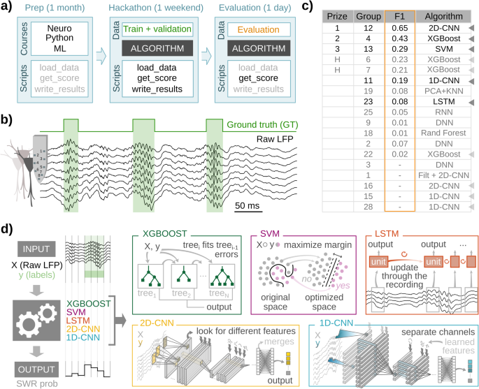
In order to explore a wide variety of ML models to the problem of SWR detection, we organized a hackathon (https://thebraincodegames.github.io/index_en.html). We specifically targeted people unfamiliar with SWR studies who could provide unbiased solutions to the challenge. A secondary goal of the hackathon was to promote their interest and engagement at the interface between Neuroscience and Artificial Intelligence, especially for future young scientists. The event was held in Madrid in October 2021, using remote web platforms. Some of us (ANO) coordinated the event. Consent to participate and to share relevant personal data was obtained prior to the event. All participants were informed of the goal of the hackathon and agreed that their solutions were subject to subsequent investigation and modification.

The hackathon comprised 36 teams of 2–5 people (71% males, 29% female), for 116 participants in total. They represent 45% of undergraduate students, 38% of master students, 15% of Ph.D. students, and 3% of non-academic workers (Supplementary Fig. 1a). On average, they were young in their professional careers, with 77% of participants being research-oriented (Supplementary Fig. 1a). Previous to the hackathon, we monitored the participants’ self-declared knowledge level on Neuroscience, Python programming, and ML, in general, using a survey (Supplementary Fig. 1b). To provide a homogeneous floor to address the challenge, we organized three online seminars to cover each of the three topics one month before the activity. Seminars were recorded and made available for review along with the experience.

The hackathon was held over one weekend (Friday to Sunday), during which groups had to design and train an ML algorithm to detect SWRs. To standardize the different algorithms for future comparison, they were given Python functions to load the data, compute a performance score, and write results in a common format. Data sets were available from a public research-oriented repository at Figshare (https://figshare.com/projects/cnn-ripple-data/117897). Participants were given a training set to train their algorithms and a validation set to run tests.

Data consisted of raw 8-channel LFP signals from the hippocampal CA1 region, recorded with high-density probes, which were used before for similar purposes30. SWR was manually tagged to be used as ground truth (training set: 1794 events, two sessions from two mice; validation set: 1275 events; two sessions from two animals). Since participants had two days to design and train solutions, groups were allowed to interact with us to ask for technical questions and clarification.

We monitored participant’s engagement throughout the hackathon using short questionnaires. This allowed us to check their motivation and other emotional states (i.e., frustration, interest, etc…). Some people dropped out during the days of the hackathon (Supplementary Fig. 1d). We found many participants felt confused and frustrated with the challenge, and this correlated with their performance, as a posterior analysis suggested (Supplementary Fig. 1e).

Training, validation, and test datasets, and ground truth

Participants of the hackathon were provided with an annotated dataset consisting of raw LFP signals recorded from head-fixed mice using high-density probes (8 channels)30. Awake SWR events were manually tagged by an expert who identified the start and the end of each event. The start of the SWR was defined near the first ripple of the sharp-wave onset. The end of the event was defined at the latest ripple or when the sharp wave resumed. The training set consisted of two recording sessions from 2 mice30. They contained 1794 manually tagged SWRs. The validation set consisted of two recording sessions from another 2 mice and contained 1275 SWR events (Supplementary Table 1).

For posterior analysis of the results of the hackathon, we used an additional test dataset consisting of the 2 validation sessions mentioned before plus another 19 sessions for a total of 21 sessions from 8 different mice. They all contained a total of 7423 manually tagged SWRs (Supplementary Table 1). In addition, to evaluate the effect of different expert’s definitions of SWRs, we used the ground-truth dataset tagged by a new expert (nGT) to compare against the original GT (oGT) used for training.

To test the ability of the trained models to detect SWR in different physiological conditions, we used data from freely moving mice recorded during awake and sleep conditions, as reported recently14. This data consisted of LFP signals obtained with linear silicon probes (16 channels) from 2 mice (Supplementary Table 1). Signals were sampled around the CA1 cell body layer and expanded by interpolation to meet the 8-channel input of the ML models (Supplementary Fig. 4e). SWR was tagged by the original expert.

ML models specifications

Five architectures were selected out of the 18 solutions submitted to the hackathon: XGBoost, SVM, LSTM, 2D-CNN, and 1D-CNN. For the purpose of fair comparisons, they were retrained and tested using homogenized pre-processing steps and data management strategies (see below).

We used Python 3.9.13 with libraries Numpy 1.19.5, Pickle 4.0, and H5Py 3.1.0. To build the different neural networks, we used the Tensorflow 2.5.3 library, with Keras 2.5.0 as the application programming interface. XGBoost 1.6.1 was used to train and test the boosted decision tree classifiers. Scikit-learn 1.1.2 and Imbalanced-learn 0.9.1 were used to train support vector machine classifiers. Analysis and training of the models were conducted on a personal computer (i7-11800H Intel processor with 16 GB RAM and Windows 10).

Data preparation

For subsequent training and analysis of the architectures selected from the hackathon, all data was pre-processed. From each recording session, two matrices were extracted: X, with the raw LFP data, shaped (# of timestamps, # of channels), and Y, the ground truth generated from the expert tagging (# of timestamps). A timestamp of Y is 1 if a SWR event is present.

Values for matrix X were subsampled at 1250 Hz, taking into consideration that SWRs are events that have frequencies in the range of up to 250 Hz. Before retraining the algorithms, data was z-scored with the mean and standard deviation of the whole session.

Training and validation split

For retraining the architectures, the same training dataset provided in the hackathon was used (2 sessions from 2 mice; 1794 SWR events). For initial testing, these two sessions were split according to a 70/30 train/validation design. To evaluate the generalization capabilities of the models when presented with unseen data, we used several test sessions, which provide the necessary animal-to-animal, as well as within-animal (sessions) variability. Test sessions included the 2 sessions from the validation dataset provided in the hackathon and 19 additional sessions (21 sessions from 8 mice, 7423 SWR events).

For re-training, the two training sessions were concatenated and divided into 60 s epochs. Each epoch was assigned randomly to the train or validation set, following the desired split proportion. The data was reshaped to be compatible with the required input dimensionality of each architecture (see below). In order to evaluate model performance, two different datasets were used: the validation set described above (used for an initial screening of the 50 best models for each architecture) and the test set (used for generalization purposes).

Identification of SWR events in the data was implemented using analysis windows of different sizes. To identify SWR events detected by the ML models, we set a probability threshold to identify windows with positive and negative predictions. GT was annotated in the different analysis windows of each session. Accordingly, predictions were classified into four categories: True Positive (TP), when the prediction was positive and the GT window did contain an SWR event; False Positive (FP), when the prediction was positive in a window that did not contain any SWR; False Negative (FN), when the prediction was negative in a window with an SWR; and True Negative (TN) when the prediction was negative and the window did not contain any SWR event.

If a positive prediction had a match with any window containing a SWR, it was considered a TP, or it was classified as FP otherwise. All true events that did not have any matching positive prediction were considered FN. Negative predictions with no matching true events windows were TN.

With predicted and true events classified into those four categories, there are three measures that can be used to evaluate the performance of the model. Precision (P), which was computed as the total number of TPs divided by TPs and FPs, represents the percentage of predictions that were correct.

$${{{{{\rm{Precision}}}}}}=\frac{{{{{\rm{TP}}}}}}{{{{{\rm{TP}}}}}+{FP}}$$

Recall (R), which was calculated as TPs divided by TPs and FNs, represents the percentage of true events that were correctly predicted.

$${{{{{\rm{Recall}}}}}}=\frac{{{{{\rm{TP}}}}}}{{{{{\rm{TP}}}}}+{FN}}$$

Finally, the F1-score, calculated as the harmonic mean of Precision and Recall, represents the network performance, penalizing imbalanced models.

$$F1=\frac{2* \left({{{{{\rm{Precision}}}}}}* {{{{{\rm{Recall}}}}}}\right)}{{{{{\rm{Precision}}}}}+{Recall}}$$

To ease subsequent evaluation of ML models for SWR analysis, we provide open access to codes for retraining strategies39: https://github.com/PridaLab/rippl-AI.

Parameter fitting

Different combinations of parameters and hyper-parameters were tested for each architecture during the training phase (1944 for XGBoost, 72 for SVM, 2160 for LSTM, 60 for 2D-CNN, and 576 for 1D-CNN).

Two parameters were shared across all architectures: the number of channels and the number of timestamps in the analysis window (referred to as the window size). These parameters define the dimensionality of the input data (# timesteps × # channels), i.e., the number of input features.

The number of channels to be used was set at 1, 3, or 8. When 1 channel was chosen, it was that corresponding to the CA1 pyramidal layer channel, defined as the channel with the most power in the ripple bandwidth (150–250 Hz). The superficial, pyramidal, and deep channels were used as 3 channels. All the channels in the shank were used for the 8-channel input configuration.

The number of timestamps defines the window size. The tested values depended on each architecture and ranged between windows of 0.8–51.2 milliseconds. The rest of the parameters were specific for each architecture (see below).

The F1-score metric for the training and validation set was calculated to compare the performance of the models, with the validation F1 serving as a priori metric of the generalization of the models, allowing for a selection of models without performing a complete test.

For each model, a test-F1 array was calculated with different thresholds (generally, from 0.1 to 0.9 with 0.1 increments), and the highest value for each model was used for comparison among models of the same architecture. As a result, the 50-best performing models were selected after the initial retrained test.

Validation process

The aim of validation is to find the model that generalizes best to unseen data for each architecture. With that in mind, defining a metric that takes this into account is not a straightforward task.

To weigh each validation session (21) independently, an F1 array was calculated for each individual session, resulting in a matrix of 21 per number of threshold values (#th). The mean of sessions gives us a #th array that quantifies the performance/generalization of the model as a function of the chosen threshold. The maximum value of this array will represent the best performance that could be achieved with this model if the threshold is correctly selected. This single value is what will be compared. Using this strategy, we narrowed down available models to the 10 best of each architecture before selecting the best model.

XGBoost

Based in the Gradient Boosting Decision Trees algorithm, this architecture trains a tree with a subset of samples and then calculates its output44. The misclassified samples are used to train a new tree. The process is repeated until a predefined number of classifiers are trained. The final model output is the weighted combination of individual outputs.

In the training process, we worked with quantitative features (LFP values per channel), and a threshold value for a specific feature was considered in each training step. If this division correctly classifies some samples of the subset, two new nodes are generated in the next tree level, where the operation is repeated until the maximum tree depth is achieved, and a new tree with the misclassified samples is generated. The input is one dimensional (# of channels × # of timesteps) and produces a single output.

Specific parameters of XGBOOST are the Maximum depth and the maximum levels for each tree, which may lead to overfitting. Learning rate, which controls the influence of each individual model in the ensemble of trees. Gamma is the minimum loss reduction required to make a further partition on a leaf node, with larger values leading to conservative models. Parameter λ contributes to the regularization, with larger values preventing overfitting. Scale is used in imbalanced problems; the larger the more penalized false negatives are during training.

Trained models had a number of trainable parameters ranging from 1500 to 17,900.

SVM

A support vector machine is a classical classifier that searches for a hyperplane in the input dimensionality that maximizes the separation between different classes. This is only possible in lineal separation problems, so some misclassifications are permitted in real tasks. Usually, SVM performs a transformation on the original data using a kernel (linear or otherwise) that increases the data dimensionality but facilitates classification.

During training, the parameters that define the separation hyperplane are updated until the maximum number of iterations is achieved or the rate of change in the parameters go below a threshold. The input is one-dimensional (# of channels × # of timesteps) and produces a single output.

Specific parameters of SVM are the kernel type. Using nonlinear kernels resulted in an explosive growth in training and predicting times due to the enormous number of training data points. Only the linear kernel produced manageable times. The under-sample proportion rules out negative samples (windows without ripple) until the desired balance is achieved: 1 indicates the same number of positives and negatives.

Trained models had a number of trainable parameters ranging from 1 to 480.

LSTM

Recurrent neural networks (RNNs) are a subtype of NNs especially suited to work with temporal series of data, extracting the hidden relations and tendencies between non-contiguous instants. Long short-term memory (LSTMs) are RNNs with modifications that prevent some associated problems46.

During training, three sets of weights and biases are updated in each LSTM unit, associated with different gates (Forget, input, and output). To prevent overfitting, two layers of dropout (DP) and batch normalization (batchNorm) were inserted between LSTM layers. DP randomly prevents some outputs from propagating to the next layer. BatchNorm normalizes the output of the previous layer. The final layer is a dense layer that outputs the event probability. The input is two-dimensional (# of timesteps, # of channels) and produces a probability for each timestep. After each window, the internal weights are reset.

Specific LSTM parameters: bidirectional if the model processes the windows forwards and backward simultaneously; # of layers is the number of LSTM layers; # of units is the number of LSTM units in each layer, and # of epochs, which is the number of times the training data is used to perform training.

Trained models had a number of trainable parameters ranging from 156 to 52851.

2D-CNN

Convolutional neural networks use convolutional layers consisting of kernels (spatial filters) to extract the relevant features of an image49. Successive layers use this as inputs to compute general features of the image. This 2D-CNN moves the kernels along the two axes, temporal (timesteps) and spatial (channels). The first half of the architecture includes MaxPooling layers that reduce the dimensionality and prevent overfitting. A batchNorm layer follows every convolutional layer. Finally, a dense layer produces the event probability of the window.

During training, the weights and biases of every kernel are updated to minimize the loss function, which was taken as the binary cross entropy:

$${H}_{p}\left(q\right)=\frac{-1}{N}\mathop{\sum }\limits_{i=1}^{N}{y}_{i}\cdot \log \left(p\left({y}_{i}\right)\right)+\left(1-{y}_{i}\right)\cdot \log \left(1-p\left({y}_{i}\right)\right)$$

N is the number of windows in the training set, yi is the label of the i window and p(yi) is the probability of ripple that the model predicts. The input is # of timesteps and # of channels; and produces a single probability for each window.

The 2D-CNN was tested with a fixed number of layers and kernel dimensions. The kernel factor parameter determined the number of kernels in this structure: 32 × kf (2 × 2), 16 × kf (2 × 2), 8 × kf (3 × 2), 16 × kf (4 × 1), 16 × kf (6 × 1), and 8 × kf (8 × 1). In parenthesis, the size of the kernels in each layer.

Trained models had a number of trainable parameters ranging from 1713 to 24,513.

1D-CNN

This model is also a convolutional neural network, but the kernels only move along the temporal axis while processing spatial information. The number of layers and the kernel size were fixed. The tested models had 7 sets of 1D convolutional layer, batchNorm, and LeakyRelu layer, followed by a dense sigmoid activation unit. This model is similar to our previous CNN solution30.

During training, the weights and biases of the layers were also updated with the objective of minimizing the binary cross entropy. The input is # of timesteps and # of channels and produces a single probability for each window.

The specific parameters for 1D-CNN included the kernel factor, which defined the number of kernels in each conv layer. The size and stride for each layer were equal and fixed. The size of the kernels in the first layer was defined as the length of the input window divided by 8. Structure: 4 × kf (# timesteps//8 × # timesteps//8), 2 × kf (1 × 1), 8 × kf (2 × 2), 4 × 1 (1 × 1), 16 × kf (2 × 2), 8 × kf (1 × 1), and 32 × kf 2 × 2). Parameters also include # of epochs, the number of times the training data is used to perform training, and # of training batch samples, which is the number of windows that are processed before parameter updating.

Trained models had a number of trainable parameters ranging from 342 to 4253.

Filter

We used a Butterworth filter, which is considered the gold standard for SWR detection25. The parameters that we varied were the high-cut frequency, the low-cut frequency, and the filter order. No training was run, but instead, all combinations between parameters were tested, and the best 10 models were kept. The 10 best models had the following set of parameters: (1) 100–250 Hz and 5th order, (2) 100–250 Hz 4th order, (3) 100–250 Hz 8th order, (4) 100–250 Hz 7th order, (5) 100–250 Hz 6th order, (6) 100–250 Hz 3rd order, (7) 100–250 Hz 9th order, (8) 100–250 Hz 10th order, (9) 100–250 Hz 2nd order, (10) 90–250 Hz 5th order.

In order to extract the event times using the filter output, the envelope of the filtered signal is computed. The standard deviation of this signal is multiplied by a factor used to define a threshold. The intervals where the filtered signal surpasses said threshold are the detected events.

Threshold alignment to compare F1 curves in Supplementary Fig. 4 was done by selecting 9 standard deviation multiplication factors that resulted in a similar F1 curve as those in the ML models: 2, 2.5, 3, 3.5, 4, 4.5, 5, 5.5, 6, 6.5, and 7.

Ensemble model

This model consists of a single-layer perceptron, with 5 inputs and 1 output, computed using a sigmoid as the activation function. It takes the predicted output of the previously trained ML models and combines them in a weighted probability.

During training, the weights and biases of the layer were updated with the objective of minimizing the binary cross entropy. The input shape is 5 (the output of the models) and generates a probability for each timestamp.

Parameters tested during training were the number of epochs and the number of samples per training batch. This trained model had 6 trainable parameters: 5 weights and 1 bias.

Stability index

This metric, shown in Fig. 4c, quantifies the consistency of the performance of a model across all possible thresholds. It is calculated as the number of thresholds whose F1 is above the 90% of the best F1 value of the model divided by the total number of thresholds.

Possible metric values range from 1, from a very consistent model, and 0, from a completely inconsistent model.

Characterization of SWR features

SWR properties (ripple frequency and power) were computed using a 100 ms window around the center of the event, measured at the pyramidal channel of the raw LFP. Preferred frequency was computed first by calculating the power spectrum of the 100 ms interval using the enlarged bandpass filter 70 and 400 Hz, and then looking for the frequency of the maximum power. In order to account for the exponential power decay in higher frequencies, we subtracted a fitted exponential curve (‘fitnlm’ from MATLAB toolbox) before looking for the preferred frequency. To estimate the ripple power, the spectral contribution was computed as the sum of the power values for all frequencies lower than 100 Hz normalized by the sum of all power values for all frequencies (of note, no subtraction was applied to this power spectrum).

Dimensionality reduction using UMAP

To classify SWR, we used topological approaches14. The UMAP version 0.5.1 (https://umap-learn.readthedocs.io/en/latest/) in Python 3.8.10 Anaconda was used, which is known to properly preserve local and global distances while embedding data in a lower dimensional space. In all cases, we used default values for reconstruction parameters. Algorithms were initialized randomly. UMAP provided robust results independent of initialization. Events were GT ripples sampled at 1250 Hz, centered around the SWR trough closest to the highest SWR spectral power, and taking a 50 ms window around that point. As a result, events were points in a 63 (1 + 0.025*1250) dimensional cloud. The parameters chosen to fit the cloud were: the metric (metric) was Euclidean; the number of neighbors (n_neighbors), which controls how UMAP balances local vs global structure in the data, was set to 20; minimum distance (min_dist), which controls how tightly UMAP is allowed to pack points together by setting the minimum distance apart that points are allowed to be in the low dimensional representation, was set to 0.1; and the number of components (n_components), that sets the dimensionality of the reduced dimension space we will be embedding the data into, was set to 4. This goes in accordance with previous studies that had shown the intrinsic dimension of SWRs is 4D14.

Prediction and re-training of non-human primate data set

To study the generalization capabilities of the different architectures, we used data from a freely moving macaque targeting similar CA1, as completed in our mouse data (methods are described in ref. 54). Recordings were obtained with a 64-ch linear polymer probe (custom ‘deep array probe’, Diagnostic Biochips) that recorded across the CA1 layers of the anterior hippocampus (Fig. 6a) where layers were identifiable relative to the main pyramidal layer, which contains the greatest unit activity and SWP power. LFP signals were sampled at 30 kHz using a Freelynx wireless acquisition system (Neuralynx, Inc.). Data corresponds to periods of immobility for a duration of almost 2 h and 40 min, predominantly comprised of sleep in overnight housing.

Similar to the procedures used in mice, SWR beginning and ending times were manually tagged (ground truth). First, the best model of each architecture, already trained with the mouse data, was used to predict the output of the primate data with no retraining. For this purpose, we used recordings of different channels around the CA1 pyramidal channel, matched to meet the laminar organization of the dorsal mouse hippocampus. Specifically, we used one CA1 radiatum channel, 720 µm from the pyramidal layer, three channels in the pyramidal layer, at +90 µm, +0 µm and −90 µm from the pyramidal channel, and a stratum oriens channel 720 µm from the pyramidal channel. The pyramidal channel was defined at the site with the maximal ripple power. We complemented these 5 recordings with 3 more interpolated signals, making a total of 8 input channels [oriens, interpolated, pyramidal, pyramidal, pyramidal, interpolated, interpolated, radiatum] using a linear interpolation script available at Github: https://github.com/PridaLab/rippl-AI/blob/main/aux_fcn.py. The applied pre-processing was the same as with the mice data: subsampling to 1250 Hz and z-score normalization.

With the aim of studying the effect of retraining with completely different data, we retrained the models. Data was split in three sets (50% training, 20% validation, 30% test), and used to retrain and validate the models. For re-training, we reset all trainable parameters (internal weights) but kept all architectural hyper-parameters fixed (input number of channels, input window length, number of layers, etc…) as with the mouse data, making the re-training process much faster than the original training that required a deep hyper-parametric search (per model re-train: 2 min for XGBoost, 10–30 min for SVM, 3–20 min for LSTM, 1–10 min for 2D-CNN and 1–15 min for 1D-CNN). We used a second expert tagging to evaluate the generalization capability of retrained models.

Statistics and reproducibility

Statistical analysis was performed with Python and/or MATLAB. Kruskal–Wallis tests were applied for group analysis. Post hoc comparisons were evaluated with Tukey–Kramer two-tailed tests with appropriate adjustments for multiple comparisons. In most cases, values were z-scored (subtract the mean from each value and divide the result by the s.d.) to make data comparable between experimental sessions and across layers. Reproducibility was tested in several experimental sessions, with the number of replications specified.